Article for Journal of Open Source Software

Martin Vonk (2025)

This notebook replicates the results presented in the article submitted to the Journal of Open Source Software (JOSS). The article can be found here: Vonk, M. A. (2025). SPEI: A Python package for calculating and visualizing drought indices. Journal of Open Source Software, 10(111), 8454. doi.org/10.21105/joss.08454

JOSS is a developer-friendly, open-access academic journal (ISSN 2475-9066) dedicated to research software packages and features a formal peer-review process. The pre-review and review of the SPEI package are publicly available in issues openjournals/joss-reviews#8430 and openjournals/joss-reviews#8454, respectively.

Setup

# dependencies
from typing import Literal

import matplotlib as mpl
import matplotlib.pyplot as plt
import numpy as np
import pandas as pd
import scipy.stats as sps
from cycler import cycler
from matplotlib import patheffects
from scipy.stats._survival import EmpiricalDistributionFunction

import spei as si

# matplotlib settings
plt.rcParams.update(
    {
        "axes.prop_cycle": cycler(
            color=[
                "#3f90da",
                "#ffa90e",
                "#bd1f01",
                "#94a4a2",
                "#832db6",
                "#a96b59",
                "#e76300",
                "#b9ac70",
                "#717581",
                "#92dadd",
            ]
        ),
        "axes.titlesize": 7.0,
        "axes.labelsize": 7.0,
        "xtick.labelsize": 6.0,
        "ytick.labelsize": 6.0,
        "legend.fontsize": 7.0,
        "legend.framealpha": 1.0,
    }
)


# helper functions
def axes_indicator(
    ax: plt.Axes,
    letter: str,
    x: float,
    y: float,
    ha: Literal["left", "right"],
    va: Literal["top", "bottom"],
):
    """Add an indicator to the axes."""
    ax.annotate(
        f"({letter})",
        xy=(x, y),
        xycoords="axes fraction",
        fontsize=mpl.rcParams["axes.titlesize"],
        horizontalalignment=ha,
        verticalalignment=va,
        path_effects=[
            patheffects.Stroke(linewidth=1, foreground="white"),
            patheffects.Normal(),
        ],
    )


def plot_ecdf(
    ax: plt.Axes,
    data: pd.Series,
    ecdf: EmpiricalDistributionFunction,
    s: float,
    color: str,
    label: str,
    cdf: pd.Series | None = None,
    **kwargs,
) -> None:
    data = data.drop_duplicates()
    ax.scatter(
        data,
        ecdf.probabilities,
        s=s,
        facecolor=color,
        label=label,
        **kwargs,
    )
    if cdf is not None:
        for idata, icdf, iecdf in zip(data, cdf, ecdf.probabilities):
            ax.plot(
                [idata, idata],
                [iecdf, icdf],
                color=color,
                linewidth=0.5,
                **kwargs,
            )
    return ecdf

Data

Load

df = pd.read_csv("data/CABAUW.csv", index_col=0, parse_dates=True)
prec = df["prec"]
evap = df["evap"]
surplusd = prec - evap
surplus = surplusd.resample("MS").sum()
head = df["head"]

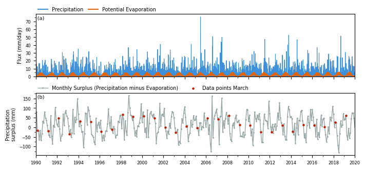
Plot

# highlight specific month
month = 3
ts = pd.Timestamp("2000-{:02d}-01".format(month))

fig, axd = plt.subplot_mosaic(
    [["meteo"], ["sp"]], figsize=(7.0, 3.2), sharex=True, layout="constrained"
)

axd["meteo"].plot(prec.index, prec, linewidth=0.8, color="C0")
axd["meteo"].plot(evap.index, evap, linewidth=0.8, color="C6")
axd["meteo"].plot([], [], color="C0", label="Precipitation")
axd["meteo"].plot([], [], color="C6", label="Potential Evaporation")

axd["meteo"].legend(loc=(0, 1), ncol=2, frameon=False, columnspacing=1.0)
axd["meteo"].set_ylabel("Flux (mm/day)")

axd["meteo"].yaxis.set_major_locator(mpl.ticker.MultipleLocator(10))
axd["meteo"].yaxis.set_minor_locator(mpl.ticker.MultipleLocator(5))
axd["meteo"].set_ylim(bottom=0.0)
axes_indicator(axd["meteo"], letter="a", x=0.005, y=0.97, ha="left", va="top")

axd["sp"].plot(
    surplus.index,
    surplus.values,
    color="C3",
    linewidth=1.0,
    marker=".",
    markersize=2.0,
    label="Monthly Surplus (Precipitation minus Evaporation)",
)
mid = surplus.index.month == ts.month
axd["sp"].scatter(
    surplus.index[mid],  # + pd.Timedelta(days=15),
    surplus.values[mid],
    color="C2",
    s=5.0,
    zorder=2,
    label=f"Data points {ts.strftime('%B')}",
)
axd["sp"].yaxis.set_major_locator(mpl.ticker.MultipleLocator(50))
axd["sp"].yaxis.set_minor_locator(mpl.ticker.MultipleLocator(25))
axd["sp"].xaxis.set_minor_locator(mpl.dates.YearLocator(1))
axd["sp"].xaxis.set_major_locator(mpl.dates.YearLocator(2))
axd["sp"].set_xlim(surplus.index[0], surplus.index[-1])
axd["sp"].set_ylabel("Precipitation\nsurplus (mm)")
axd["sp"].legend(loc=(0, 1), frameon=False, ncol=2)
axes_indicator(axd["sp"], letter="b", x=0.005, y=0.97, ha="left", va="top")

axd["sp"].set_xlim(pd.Timestamp("1990"), pd.Timestamp("2020"))

# fig.savefig("../../paper/figures/monthly_precipitation_surplus.png", dpi=300, bbox_inches="tight")

(np.float64(7305.0), np.float64(18262.0))

Standardized Index Procedure

Fit Distribution

dist = sps.fisk
sispei = si.SI(
    series=surplus,
    dist=dist,
    timescale=1,
    # fit_freq="MS",
)
sispei.fit_distribution()

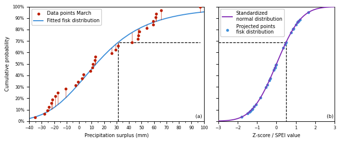
Equiprobability Transform

fit_dist = sispei._dist_dict[ts]
data = fit_dist.data.sort_values()
cdf = fit_dist.cdf().loc[data.index]
ecdf = sps.ecdf(data).cdf

zscores = np.arange(-3.0, 3.1, 0.1)
norm_cdf = sps.norm.cdf(zscores, loc=0.0, scale=1.0)
norm_cdf_transformed = sps.norm.ppf(cdf.values, loc=0.0, scale=1.0)

fig, axd = plt.subplot_mosaic(
    [["cdf", "norm"]],
    figsize=(7.0, 3),
    width_ratios=[1.5, 1.0],
    sharey=True,
    layout="tight",
)
plot_ecdf(
    ax=axd["cdf"],
    data=data,
    cdf=cdf,
    ecdf=ecdf,
    s=10.0,
    color="C2",
    label=f"Data points {ts.strftime('%B')}",
    zorder=3,
)

bin = 5.0
bins = np.arange(data.min() // bin * bin, data.max() + bin, bin)
axd["cdf"].plot(
    bins,
    fit_dist.dist.cdf(bins, *fit_dist.pars, loc=fit_dist.loc, scale=fit_dist.scale),
    label=f"Fitted {dist.name} distribution",
    color="C0",
)

axd["cdf"].legend(loc="upper left")
axd["cdf"].set_xlim(np.min(bins), np.max(bins))
axd["cdf"].xaxis.set_minor_locator(mpl.ticker.MultipleLocator(bin))
axd["cdf"].xaxis.set_major_locator(mpl.ticker.MultipleLocator(bin * 2))
axd["cdf"].set_ylim(0.0, 1.0)
axd["cdf"].yaxis.set_major_locator(mpl.ticker.MultipleLocator(0.1))
axd["cdf"].yaxis.set_major_formatter(mpl.ticker.PercentFormatter(1.0))
axd["cdf"].set_xlabel("Precipitation surplus (mm)")
axd["cdf"].set_ylabel("Cumulative probability")
axes_indicator(axd["cdf"], "a", 0.99, 0.02, ha="right", va="bottom")

axd["norm"].plot(
    zscores, norm_cdf, label="Standardized\nnormal distribution", color="C4", zorder=3
)
axd["norm"].scatter(
    norm_cdf_transformed,
    cdf.values,
    s=10.0,
    label=f"Projected points\n{dist.name} distribution",
    color="C0",
    zorder=2,
)
axd["norm"].legend(loc="upper left")
axd["norm"].set_xlim(np.min(zscores), np.max(zscores))
axd["norm"].set_xlabel("Z-score / SPEI value")

# visualize specific data point
idx = data.index[20]
cdf_idx = cdf.at[idx]
ppf_idx = sps.norm.ppf(cdf_idx)
print(
    f"Data index: {idx.strftime('%Y')}, Data value: {data.loc[idx]:0.2f} CDF: {cdf_idx:0.1%}, PPF: {ppf_idx:0.4f}"
)
axd["cdf"].plot(
    [data.loc[idx], data.loc[idx], np.max(data)],
    [0.0, cdf_idx, cdf_idx],
    color="k",
    linestyle="--",
    linewidth=1.0,
    zorder=0,
)
axd["norm"].plot(
    [np.min(zscores), ppf_idx, ppf_idx],
    [
        cdf_idx,
        cdf_idx,
        0.0,
    ],
    color="k",
    linestyle="--",
    linewidth=1.0,
    zorder=0,
)
axes_indicator(axd["norm"], "b", 0.99, 0.02, ha="right", va="bottom")

# fig.savefig("../../paper/figures/surplus_fit_cdf.png", dpi=300, bbox_inches="tight")

Data index: 1994, Data value: 31.30 CDF: 68.9%, PPF: 0.4925

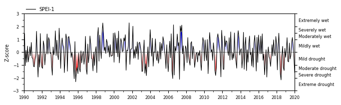
Results

Time Series

spei1 = sispei.norm_ppf()

ax = si.plot.si(spei1, figsize=(7.0, 2.0), layout="tight")
# ax.xaxis.set_minor_locator(mpl.dates.MonthLocator())
ax.xaxis.set_minor_locator(mpl.dates.YearLocator(1))
ax.xaxis.set_major_locator(mpl.dates.YearLocator(2))
ax.legend(labels=["SPEI-1"], loc=(0, 1), frameon=False)
ax.set_xlim(pd.Timestamp("1990"), pd.Timestamp("2020"))
ax.set_ylabel("Z-score")

# ax.get_figure().savefig("../../paper/figures/spei1.png", dpi=300, bbox_inches="tight")

Text(0, 0.5, 'Z-score')

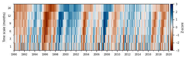
Heatmap

speis = [
    spei1.rename("1"),
    si.spei(surplus, timescale=3).rename("3"),
    si.spei(surplus, timescale=6).rename("6"),
    si.spei(surplus, timescale=9).rename("9"),
    si.spei(surplus, timescale=12).rename("12"),
    si.spei(surplus, timescale=24).rename("24"),
]
f, ax = plt.subplots(figsize=(7.0, 2.0))
si.plot.heatmap(speis, cmap="vik_r", vmin=-3, vmax=3, add_category=False, ax=ax)
ax.set_ylabel("Time scale (months)")
f.axes[-1].set_ylabel("Z-score")
ax.xaxis.set_minor_locator(mpl.dates.YearLocator(1))
ax.xaxis.set_major_locator(mpl.dates.YearLocator(2))
ax.set_xlim(pd.Timestamp("1990"), pd.Timestamp("2020"))

# ax.get_figure().savefig("../../paper/figures/spei_heatmap.png", dpi=300, bbox_inches="tight")

(np.float64(7305.0), np.float64(18262.0))

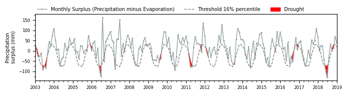
Threshold

perc = sps.norm.cdf(-1.0)  # same as zscore -1.0
thres = sispei.ppf(perc).rename(f"Threshold {perc:0.0%} percentile")
fig, ax = plt.subplots(figsize=(7.0, 2.0), layout="tight")
ax = si.plot.threshold(
    surplus,
    thres,
    ax=ax,
    **dict(
        color="C3",
        linewidth=1.0,
        marker=".",
        markersize=2.0,
        label="Monthly Surplus (Precipitation minus Evaporation)",
    ),
)
ax.set_xlim(pd.Timestamp("2003"), pd.Timestamp("2019"))
ax.yaxis.set_major_locator(mpl.ticker.MultipleLocator(50))
ax.yaxis.set_minor_locator(mpl.ticker.MultipleLocator(25))
ax.xaxis.set_major_locator(mpl.dates.YearLocator(1))
ax.xaxis.set_minor_locator(mpl.dates.MonthLocator([4, 7, 10]))
ax.set_ylabel("Precipitation\nsurplus (mm)")
ax.legend(ncol=3, loc=(0, 1), frameon=False)

# fig.savefig("../../paper/figures/threshold.png", dpi=300, bbox_inches="tight")

<matplotlib.legend.Legend at 0x7f3bcaee3710>