Package Comparison¶

Martin Vonk - 2023

This notebooks compares the calculated drought indices to other (Python) packages or time series retrieved from other locations. Current comparisons include:

standard_precip (Python)
climate_indices (Python)
pastas (Python)
SPEI (R)

Please note that it can be difficult to install these packages. SPEI (R) requires the R library. Pastas depends on Numba which has strict requirements for NumPy. Climate Indices only supports Python 3.11 and lower. Therefore running this notebook can be cumbersome.

Future comparisons:

KNMI

Required packages¶

[1]:

import matplotlib.pyplot as plt
import pandas as pd
import scipy.stats as scs

import spei as si

print(si.show_versions())

python: 3.11.13
spei: 0.8.0
numpy: 2.2.6
scipy: 1.16.1
matplotlib: 3.10.3
pandas: 2.3.1

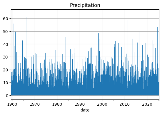
Read Precipitation Data¶

[2]:

df = pd.read_csv("data/DEBILT.csv", index_col=0, parse_dates=True)
df.index.name = "date"
prec = df["Prec [m/d] 260_DEBILT"].multiply(1e3).rename("rain")
head = df["Head [m] B32C0572_DEBILT"].rename("B32C0572").dropna()

_ = prec.plot(grid=True, linewidth=0.5, title="Precipitation", figsize=(6.5, 4))

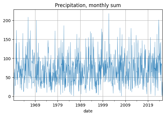
../_images/examples_example04_package_comparison_3_0.png

[3]:

# get rolling sum
prec_rsum = prec.resample("ME").sum()
_ = prec_rsum.plot(
    grid=True, linewidth=0.5, title="Precipitation, monthly sum", figsize=(6.5, 4)
)

../_images/examples_example04_package_comparison_4_0.png

Compute Standardized Precipitation Index¶

Using SPEI package¶

[4]:

spi = si.spi(prec_rsum, dist=scs.gamma, prob_zero=True, timescale=3, fit_freq="ME")
spi  # pandas Series

[4]:

date
1959-09-30   -0.859224
1959-10-31   -1.897037
1959-11-30   -2.189269
1959-12-31   -1.000515
1960-01-31   -0.231999
                ...
2025-01-31    0.272794
2025-02-28   -0.152606
2025-03-31   -1.156964
2025-04-30   -1.394517
2025-05-31   -2.469426
Freq: ME, Length: 789, dtype: float64

Using standard_precip package¶

[5]:

from standard_precip import spi as sp_spi

# standard_precip also needs rolling sum dataframe, even though you provide freq="M" and scale = 1
precdf = prec_rsum.to_frame().reset_index().copy()

# initialize spi
standardp_spi_inst = sp_spi.SPI()

# caclulate index with many parameters
standardp_spi = standardp_spi_inst.calculate(
    precdf,
    date_col="date",
    precip_cols="rain",
    freq="M",
    scale=3,  # note that scale is not the same for the standard deviation in SciPy
    fit_type="mle",
    dist_type="gam",
)
standardp_spi.index = standardp_spi.loc[
    :, "date"
].values  # create datetimeindex because date had to be a column

standardp_spi  # pandas DataFrame

[5]:

	date	rain_scale_3	rain_scale_3_calculated_index
1959-07-31	1959-07-31	NaN	NaN
1959-08-31	1959-08-31	NaN	NaN
1959-09-30	1959-09-30	79.1	-1.977699
1959-10-31	1959-10-31	102.0	-1.953337
1959-11-30	1959-11-30	110.8	-2.189269
...	...	...	...
2025-01-31	2025-01-31	253.0	0.288813
2025-02-28	2025-02-28	201.2	-0.118100
2025-03-31	2025-03-31	121.8	-1.157576
2025-04-30	2025-04-30	72.2	-1.723688
2025-05-31	2025-05-31	39.2	-2.480334

791 rows × 3 columns

Using climate_indices package¶

Previously there was a significant difference beteween the SPEI and climate_indices package, not sure why. I thought it had something to do with the fitting method used for the gamma distribution. In issue #61 it was mentioned that the same outcome could be achieved. However, I found it difficult to install climate_indces due to lack of support (for newer python versions).

[6]:

# from climate_indices.compute import scale_values, Periodicity
# from climate_indices import compute, indices, utils

[7]:

# initial_year = prec_rsum.index[0].year
# calibration_year_initial = prec_rsum.index[0].year
# calibration_year_final = prec_rsum.index[-1].year
# period_times = 366
# scale = 1
# periodicity = compute.Periodicity.daily

# values = prec_rsum.values

# scaled_values = compute.scale_values(
#     values,
#     scale=scale,
#     periodicity=periodicity,
# )

# alphas, betas = compute.gamma_parameters(
#     scaled_values,
#     data_start_year=initial_year,
#     calibration_start_year=calibration_year_initial,
#     calibration_end_year=calibration_year_final,
#     periodicity=periodicity,
# )

# gamma_params = {"alpha": alphas, "beta": betas}

# spival = indices.spi(
#     values,
#     scale=scale,
#     distribution=indices.Distribution.gamma,
#     data_start_year=initial_year,
#     calibration_year_initial=calibration_year_initial,
#     calibration_year_final=calibration_year_final,
#     periodicity=compute.Periodicity.daily,
#     fitting_params=gamma_params,
# )

# climateind_spi = pd.Series(spival, index=prec_rsum.index, name="Climate Index SPI")
# climateind_spi

Using SPEI R package¶

[8]:

from rpy2.robjects import pandas2ri
from rpy2.robjects.packages import importr

sr = importr("SPEI")

with pandas2ri.converter.context():  # pandas2ri.activate()
    spir_res = sr.spi(prec_rsum.values, scale=3)

r_spi = pd.Series(spir_res[2].ravel(), index=prec_rsum.index, name="SPI")
r_spi

/home/runner/work/SPEI/SPEI/.tox/docu/lib/python3.11/site-packages/rpy2/rinterface/__init__.py:1211: UserWarning: Environment variable "LD_LIBRARY_PATH" redefined by R and overriding existing variable. Current: "/opt/hostedtoolcache/Python/3.11.13/x64/lib", R: "/opt/R/4.3.3/lib/R/lib:/usr/local/lib:/usr/lib/x86_64-linux-gnu:/usr/lib/jvm/java-21-openjdk-amd64/lib/server:/opt/hostedtoolcache/Python/3.11.13/x64/lib"
  warnings.warn(
/home/runner/work/SPEI/SPEI/.tox/docu/lib/python3.11/site-packages/rpy2/rinterface/__init__.py:1211: UserWarning: Environment variable "LD_LIBRARY_PATH" redefined by R and overriding existing variable. Current: "/opt/R/4.3.3/lib/R/lib:/usr/local/lib:/usr/lib/x86_64-linux-gnu:/usr/lib/jvm/java-21-openjdk-amd64/lib/server:/opt/hostedtoolcache/Python/3.11.13/x64/lib", R: "/opt/R/4.3.3/lib/R/lib:/usr/local/lib:/usr/lib/x86_64-linux-gnu:/usr/lib/jvm/java-21-openjdk-amd64/lib/server:/opt/R/4.3.3/lib/R/lib:/usr/local/lib:/usr/lib/x86_64-linux-gnu:/usr/lib/jvm/java-21-openjdk-amd64/lib/server:/opt/hostedtoolcache/Python/3.11.13/x64/lib"
  warnings.warn(
/home/runner/work/SPEI/SPEI/.tox/docu/lib/python3.11/site-packages/rpy2/rinterface/__init__.py:1211: UserWarning: Environment variable "R_SESSION_TMPDIR" redefined by R and overriding existing variable. Current: "/tmp/Rtmp1fOdNB", R: "/tmp/RtmpyBt5gp"
  warnings.warn(

---------------------------------------------------------------------------
PackageNotInstalledError                  Traceback (most recent call last)
Cell In[8], line 4
      1 from rpy2.robjects import pandas2ri
      2 from rpy2.robjects.packages import importr
----> 4 sr = importr("SPEI")
      6 with pandas2ri.converter.context():  # pandas2ri.activate()
      7     spir_res = sr.spi(prec_rsum.values, scale=3)

File ~/work/SPEI/SPEI/.tox/docu/lib/python3.11/site-packages/rpy2/robjects/packages.py:472, in importr(name, lib_loc, robject_translations, signature_translation, suppress_messages, on_conflict, symbol_r2python, symbol_resolve, data)
    440 """ Import an R package.
    441
    442 Arguments:
   (...)    468
    469 """
    471 if not isinstalled(name, lib_loc=lib_loc):
--> 472     raise PackageNotInstalledError(
    473         'The R package "%s" is not installed.' % name
    474     )
    476 if suppress_messages:
    477     ok = quiet_require(name, lib_loc=lib_loc)

PackageNotInstalledError: The R package "SPEI" is not installed.

Plot and compare¶

[9]:

f, ax = plt.subplot_mosaic(
    [["SPI"], ["DIFF"]],
    figsize=(8, 4),
    sharex=True,
    height_ratios=[2, 1],
)
spi.plot(ax=ax["SPI"], grid=True, linestyle="-", label="SPI")
standardp_spi.iloc[:, -1].plot(
    ax=ax["SPI"],
    color="C1",
    grid=True,
    linestyle="--",
    label="standard_precip",
)
# climateind_spi.plot(
#     ax=ax["SPI"], color="C2", grid=True, linestyle=":", label="climate_indices"
# )
# r_spi.plot(ax=ax["SPI"], color="C2", grid=True, linestyle=":", label="R package")

(ax["SPI"].set_ylim(-3.5, 3.5),)
(ax["SPI"].set_title("Comparison"),)
(ax["SPI"].set_ylabel("SPI"),)
ax["SPI"].legend(ncol=3)

(spi - standardp_spi.iloc[:, -1]).plot(
    ax=ax["DIFF"], color="C4", label="SPEI - standard_precip", grid=True
)
# (spi - r_spi).plot(ax=ax["DIFF"], color="C3", label="SPEI - R Package")

# ax["DIFF1"].set_ylim(-0.05, 0.05)
ax["DIFF"].legend(ncol=2)
ax["DIFF"].set_title("SPEI minus other package")
ax["DIFF"].set_ylabel("Difference")
ax["DIFF"].set_xlim("1996", "1999")
f.tight_layout()

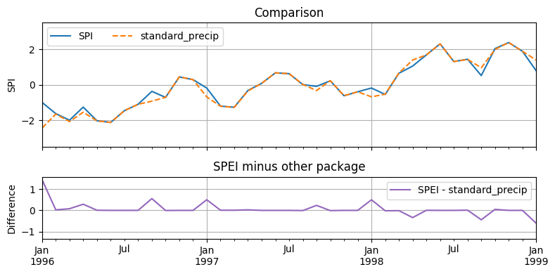
../_images/examples_example04_package_comparison_15_0.png

Difference is very small between SPEI an the standard_precip package.

The standard_precip package does not explicitely support the Standardized Precipitation Evaporation Index, as far as I can see. However, the SPI class in standard_precip could probably be used, even though the naming of precip_cols is not universal. In general, the standard_precip package needs much more keyword arguments while the SPEI package makes more use of all the nice logic already available in SciPy and Pandas.

The climate_indices package needs even more code.

The SPEI R package also has a similar result but seems to vary a bit more. More research is needed to understand why that is the case. Most likely is the differences in fitting the gamma distribution.

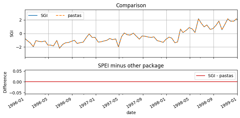
Compute Standardized Groundwater Index¶

[10]:

import pastas as ps

sgi = si.sgi(head, fit_freq="ME")
sgi_pastas = ps.stats.sgi(head)

DeprecationWarning: As of Pastas 1.5, no noisemodel is added to the pastas Model class by default anymore. To solve your model using a noisemodel, you have to explicitly add a noisemodel to your model before solving. For more information, and how to adapt your code, please see this issue on GitHub: https://github.com/pastas/pastas/issues/735

[11]:

pd.concat([sgi, sgi_pastas], axis=1).rename(columns={0: "SGI", "head": "Pastas"})

[11]:

	SGI	B32C0572
date
1968-12-13	0.510073	0.510073
1968-12-24	0.398855	0.398855
1969-01-14	0.220807	0.220807
1969-01-28	0.744936	0.744936
1969-02-14	0.650837	0.650837
...	...	...
2020-10-28	-0.052796	-0.052796
2020-11-15	-0.628006	-0.628006
2020-11-27	-0.510073	-0.510073
2020-12-14	-0.823894	-0.823894
2020-12-28	0.345126	0.345126

1225 rows × 2 columns

[12]:

f, ax = plt.subplot_mosaic(
    [["SGI"], ["DIFF"]],
    figsize=(8, 4),
    sharex=True,
    height_ratios=[2, 1],
)
sgi.plot(ax=ax["SGI"], grid=True, linestyle="-", label="SGI")
sgi_pastas.plot(ax=ax["SGI"], color="C1", grid=True, linestyle="--", label="pastas")
(ax["SGI"].set_ylim(-3.5, 3.5),)
(ax["SGI"].set_title("Comparison"),)
(ax["SGI"].set_ylabel("SGI"),)
ax["SGI"].legend(ncol=3)

(sgi - sgi_pastas).plot(ax=ax["DIFF"], color="C3", label="SGI - pastas")

ax["DIFF"].legend(ncol=2)
ax["DIFF"].set_title("SPEI minus other package")
ax["DIFF"].set_ylabel("Difference")
ax["DIFF"].set_xlim("1996", "1999")
f.tight_layout()

../_images/examples_example04_package_comparison_20_0.png