Pedotransfer Functions

Martin Vonk (2025)

Overview

Pedotransfer functions (PTFs) are empirical relationships that estimate soil hydraulic parameters from easily measured soil properties. They solve a practical problem: direct measurement of soil hydraulic properties is expensive and time-consuming, but soil particle size distribution and bulk density are relatively quick to measure.

pedon implements multiple pedotransfer functions from the literature, allowing you to estimate soil hydraulic parameters when:

• Particle size distribution (sand, silt, clay percentages) is known

• Bulk density and organic matter content are available

• Only limited data has been measured

This notebook demonstrates several PTF methods and shows how their predictions compare.

import matplotlib.pyplot as plt

import pedon as pe

Creating a Soil Sample

To use pedotransfer functions, we first create a SoilSample with measured soil properties. Let’s use a typical loamy soil with moderate sand content.

# create soil sample
sand_p = 50  # sand [%]
silt_p = 20  # silt [%]
clay_p = 30  # clay [%]
rho = 1.5  # bulk density [g/cm3]
om_p = 10  # organic matter [%]
m50 = 150  # median sand fraction [um]
ts = False  # topsoil boolean

ss = pe.SoilSample(
    sand_p=sand_p, silt_p=silt_p, clay_p=clay_p, rho=rho, om_p=om_p, m50=m50
)

Available Pedotransfer Functions

pedon provides several PTF options. Each has different input requirements and outputs. Apply one or more PTFs to see predictions.

# wosten pedotransfer function (van Genuchten)
wos = ss.wosten(ts=ts)

# wosten pedotransfer function for sand (van Genuchten)
woss = ss.wosten_sand(ts=ts)

# wosten pedotransfer function for clay (van Genuchten)
wosc = ss.wosten_clay()

# cosby pedotransfer function (Brook-Corey)
cosb = ss.cosby()

# rosetta database (options between version 1, 2 and 3)
ros = ss.rosetta(version=3)

---------------------------------------------------------------------------
ModuleNotFoundError                       Traceback (most recent call last)
File ~/work/pedon/pedon/.tox/docu/lib/python3.11/site-packages/pedon/soil.py:434, in SoilSample.rosetta(self, version)
    433 try:
--> 434     from httpx import post as httpx_post
    435 except ImportError:

ModuleNotFoundError: No module named 'httpx'

During handling of the above exception, another exception occurred:

ImportError                               Traceback (most recent call last)
Cell In[3], line 14
     11 cosb = ss.cosby()
     13 # rosetta database (options between version 1, 2 and 3)
---> 14 ros = ss.rosetta(version=3)

File ~/work/pedon/pedon/.tox/docu/lib/python3.11/site-packages/pedon/soil.py:436, in SoilSample.rosetta(self, version)
    434     from httpx import post as httpx_post
    435 except ImportError:
--> 436     raise ImportError(
    437         "httpx is required for the rosetta method to make api calls. "
    438         "Please install it with 'pip install httpx'."
    439     )
    441 soildata = [
    442     self.sand_p,  # %
    443     self.silt_p,  # %
   (...)    447     -9.9 if self.th1500 is None else self.th1500,  # [-]
    448 ]
    450 data = {"soildata": [soildata]}

ImportError: httpx is required for the rosetta method to make api calls. Please install it with 'pip install httpx'.

# More extensive plot method
f, axs = plt.subplots(1, 2, figsize=(8, 6), sharey=True, layout="tight")

pe.plot_swrc(wos, ax=axs[0], label="Wosten")
pe.plot_swrc(woss, ax=axs[0], label="Wosten Sand")
pe.plot_swrc(wosc, ax=axs[0], label="Wosten Clay")
pe.plot_swrc(cosb, ax=axs[0], label="Cosby")
pe.plot_swrc(ros, ax=axs[0], label="Rosetta")

axs[0].set(
    yscale="log",
    title="Soil Water Retention Curve",
    xlabel="\N{GREEK SMALL LETTER THETA} [-]",
    xlim=(0, 0.5),
    ylabel="|\N{GREEK SMALL LETTER PSI}| [cm]",
)
axs[0].legend(loc="lower left")


pe.plot_hcf(wos, ax=axs[1], label="Wosten")
pe.plot_hcf(woss, ax=axs[1], label="Wosten Sand")
pe.plot_hcf(wosc, ax=axs[1], label="Wosten Clay")
pe.plot_hcf(cosb, ax=axs[1], label="Cosby")
pe.plot_hcf(ros, ax=axs[1], label="Rosetta")

axs[1].set(
    yscale="log",
    xscale="log",
    title="Hydraulic Conductivity Function",
    xlabel="Ks [cm/d]",
    xlim=(1e-10, 1e3),
)
axs[1].legend(loc="lower left")

---------------------------------------------------------------------------
NameError                                 Traceback (most recent call last)
Cell In[4], line 8
      6 pe.plot_swrc(wosc, ax=axs[0], label="Wosten Clay")
      7 pe.plot_swrc(cosb, ax=axs[0], label="Cosby")
----> 8 pe.plot_swrc(ros, ax=axs[0], label="Rosetta")
     10 axs[0].set(
     11     yscale="log",
     12     title="Soil Water Retention Curve",
   (...)     15     ylabel="|\N{GREEK SMALL LETTER PSI}| [cm]",
     16 )
     17 axs[0].legend(loc="lower left")

NameError: name 'ros' is not defined

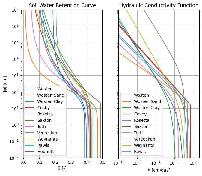
The plots above compare the predictions of different PTFs. Notice how different methods can give quite different results, particularly for the hydraulic conductivity function. This highlights the uncertainty inherent in PTFs and the importance of validating with measured data when possible.

Next Steps

If you have measured data (water retention or conductivity values), proceed to the Curve Fitting notebook to refine these estimates. If you only have a single measurement (e.g., saturated conductivity), try the HYPAGS notebook for parameter estimation from limited data.